With the understanding gained from the Introduction to 360-Degree Videos and Imaging, Open Source code can be found and evaluated for how well it supports converting equirectangular images to rectilinear images and assessed on how optimized the code appears to be. This installment in the blog series investigates several implementations and slightly modifies the code to report the length of time each algorithm takes to extract a rectilinear image.
For small projects that occasionally need to present a field of view from an equirectangular image, most any implementation works. However, code efficiency becomes far more important when the equirectangular frames are from a video or where many still images are being displayed from a sequence of images taken around the same time.
Situations exist where a single computer may handle multiple, simultaneous streams of 360-degree view images and/or videos. For instance, some security monitoring solutions may display multiple feeds simultaneously. Likewise, virtual Telesitting solutions in a hospital can display between 1 and 16 rooms on a single monitor. In these situations, having a highly optimized solution where one server can keep up with many inbound streams is paramount.
The basic steps taken by the algorithms include the following steps for each pixel in the rectilinear image:
The first code considered originates from https://github.com/rfn123/equirectangular-to-rectlinear/tree/master. The author, rfn123, notes that the code intends to assist in understanding the theory rather than producing highly efficient code. The README provides a nice explanation for the algorithm implementation and references a book for further details. This code base was forked into https://github.com/intel-health/equirectangular-to-rectlinear to add the code to report timing information. The fork also removes the YAML configuration to reduce dependencies on other code and selects some known values.
The package includes a sample 360 image to use when testing, but for this blog series, all code was minimally altered to use the same images for consistency. The two selected images are shown in Figure 1 and Figure 13 from the initial blog post. The Equirectangular to Rectilinear code depends on OpenCV for reading and writing image files and some additional operations. The original code also has a dependency on libyaml-cpp-dev since the configuration file uses YAML to define all the desired parameters, such as pan, roll, and tilt angles; however, the core algorithm does not require YAML so it can be reused elsewhere without the YMAL dependency. The framework introduced later in this series leverages that to incorporate this algorithm alongside other options.
The source code uses cmake, which reduces effort in porting to different environments. After going through the steps described in the README.md file, the code runs great and produces the expected output.
While the original author's goal concentrated on obtaining a rectilinear image and not on efficiency, the work described in this blog series attempts to produce rectilinear images efficiently. Determining the efficiency of different algorithms requires a metric to assess the speed of each. Two minor modifications were made to the code base. The first modification adds the chrono include at the top of the Equi2Rect.cpp file.
#include <chrono>
Next, as shown below, the method save_rectlinear_image was updated to utilize the high_resolution_clock for taking time measurements and added a loop around the bilinear_interpolation call. The loop allows an average time for each iteration to be calculated, which helps smooth out any impact from being swapped out of the CPU. In this case, the code ran for 100 iterations.
    std::chrono::high_resolution_clock::time_point startTime = std::chrono::high_resolution_clock::now();
    int iterations = 100;

    for (int i = 0; i < iterations; i++)
    {
        viewport.pan_angle = i % 360;
        this->bilinear_interpolation();
    }
    std::chrono::high_resolution_clock::time_point stopTime = std::chrono::high_resolution_clock::now();
    std::chrono::duration<double> aveDuration = std::chrono::duration<double>(stopTime - startTime) / iterations;
    printf("Average for %d iterations %12.8fs %12.5fms %12.3fus\n", iterations, aveDuration, aveDuration * 1000.0, aveDuration * 1000000.0);
The box below shows the results from running the code on an Intel® i9-9900k machine configured with:
Gigabyte* Desktop Board Z390 Aorus Ultra
Processor Intel(R) Core(TM) i9-9900K CPU @ 3.60GHz
Installed RAM 16.0 GB (15.9 GB usable)
System Type 64-bit operating system, x64-based processor
Intel oneAPI Base Toolkit 2023.2
Microsoft* Visual Studio 2022
First, the code was compiled and run using Debug mode. The second set of results are from running the code in Release mode. Not surprisingly, the Debug code runs slower due to additional code checks, such as range-checking method input parameters or ensuring no access to memory beyond the end of an array, which assists a developer when creating the code. The Release mode removes these checks since, presumably, the code functions properly after debugging. However, given the large difference in execution times, performance testing should use the Release mode code.
Debug\equi2rect_example.exe # Original code Debug mode
Average for 100 frames   7.23385034s   7233.85034ms  7233850.339us   0.13823897 FPS

Release\equi2rect_example.exe # Original code Release mode
Average for 100 frames   1.11301293s   1113.01293ms  1113012.927us   0.89846216 FPS
Another interesting implementation comes from https://github.com/fuenwang/Equirec2Perspec. This code uses the Python language for implementation and OpenCV to read the image and perform image operations. As with the C++ code above, the author of the Python code nicely encapsulates the core algorithm in a class. The Github ReadMe.md file shows a sample usage of that function. This code base was forked into https://github.com/intel-health/Equirec2Perspec to add the code to report timing information. A new file, RunEquirec2Perspec.py, implements the timing portion and calls an instance of the original Equirectangular class.
To instrument the code with timing information, the sample usage was augmented as follows:
import os
import cv2
import Equirec2Perspec as E2P
import time

if __name__ == '__main__':
    equ = E2P.Equirectangular('src/IMG_20230629_082736_00_095.jpg')    # Load equirectangular image

    iterations = 100
    start_time = time.perf_counter()
    for i in range(0, iterations, 1):
        #
        # FOV unit is degree
        # theta is z-axis angle(right direction is positive, left direction is negative)
        # phi is y-axis angle(up direction positive, down direction negative)
        # height and width is output image dimension
        #
        img = equ.GetPerspective(60, 0, 0, 540, 1080) # Specify parameters(FOV, theta, phi, height, width)

    end_time = time.perf_counter()
    aveDuration = (end_time - start_time) / iterations
    print("Average for ", iterations, " frames ", aveDuration, "s ", aveDuration * 1000, "ms ", aveDuration * 1000000, "us ", iterations / (end_time - start_time), " FPS")

    cv2.imshow("Flat View", img)
    cv2.waitKeyEx(0)
Like the C++ code additions, this code iterates 100 times, calling the GetPerspective method to average the results. Each iteration extracts the same perspective; that is, theta and phi are set to 0 for each iteration. If desired, one or both of the 0 parameters could be set to i to vary the selected perspective for each iteration; however, since the results are discarded, this would not be visible unless an additional cv2.imshow("Flat View", img) was added to the loop along with a cv2.waitKeyEx(1) to allow OpenCV to draw the image.
The time.perf_counter provides a clock with the highest available resolution, which can measure the time that passes between two subsequent calls.
The box below shows the results from running the code on the same Intel® i9-9900k machine as before. Two different Python execution environments were run. First is the standard distribution of Python. For the second, Intel maintains a distribution of Python that is optimized for Intel hardware available for free at https://www.intel.com/content/www/us/en/developer/tools/oneapi/distribution-for-python.html. This distribution has optimizations for accelerating core numerical packages, and it can extend numerical capabilities to other accelerators, such as a GPU. However, for this particular code, there is not a significant difference in the performance, most likely because this code relies more on the OpenCV infrastructure rather than the Python execution engine computing all the math operations. Fortunately, checking which distribution executes the code faster is very easy, and both distributions can be installed simultaneously on a machine.
py RunEquirec2Perspec.py # Standard distribution of Python 3.9.13
Average for  100  frames  0.08893186499999998 s  88.93186499999999 ms  88931.86499999999 us  11.244563464400528  FPS

python RunEquirec2Perspec.py # Intel distribution of Python 3.9.16
Average for  100  frames  0.084593784 s  84.593784 ms  84593.784 us  11.821199533998858  FPS
Interestingly enough, the Python code runs more than 10 times faster than the C++ code, but it also computes the results using slightly different techniques. For instance, the code extracting the rectilinear image calls cv2.remap, so it is worth exploring what makes Python more optimized than C++.
A fantastic tool, called Intel® VTune Profiler, assists developers in learning where code bottlenecks are, how memory is being used, uncovers interactions between threads, and generally helps visualize how code behaves. The Intel® oneAPI Base Toolkit (https://www.intel.com/content/www/us/en/developer/tools/oneapi/toolkits.html) includes VTune. Alternatively, a stand-alone version is available at https://www.intel.com/content/www/us/en/developer/tools/oneapi/vtune-profiler-download.html. Regardless of the selected download, the tool is free.
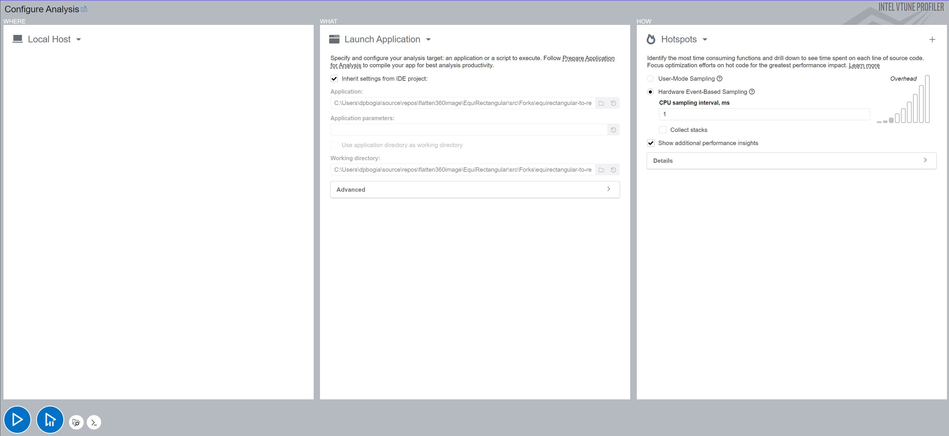
Figures 1 and 2 show the configuration used to run each program under VTune. For the C++ code, VTune was used within the Microsoft Visual Studio so all the parameters could be inherited directly from the Microsoft configuration, making it very easy to do code profiling. For the Python code, VTune was run stand-alone. Hence, VTune needed to be instructed on where to find the desired Python application, where to find the Python code to be executed, and which working directory to use while running the application.
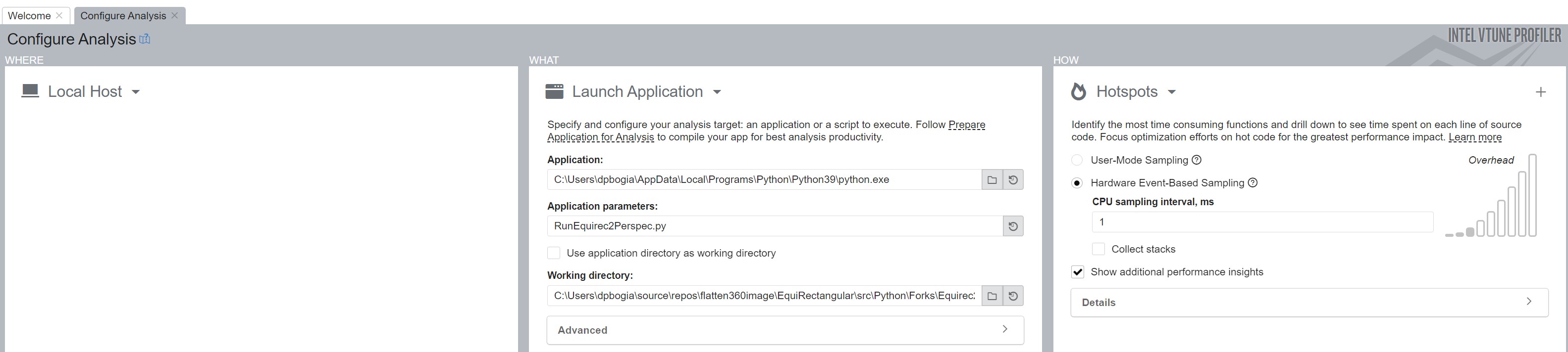
For both VTune runs, the Hotspots profiling mode was selected using hardware event sampling. This provides deeper insights into the code execution; however, it does require running VTune (or Visual Studio) with Administrator privileges.
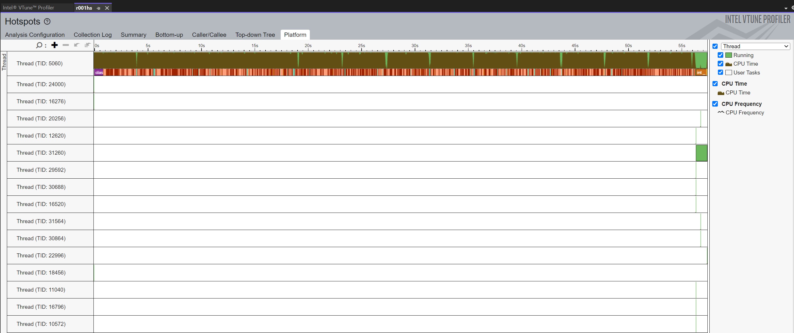
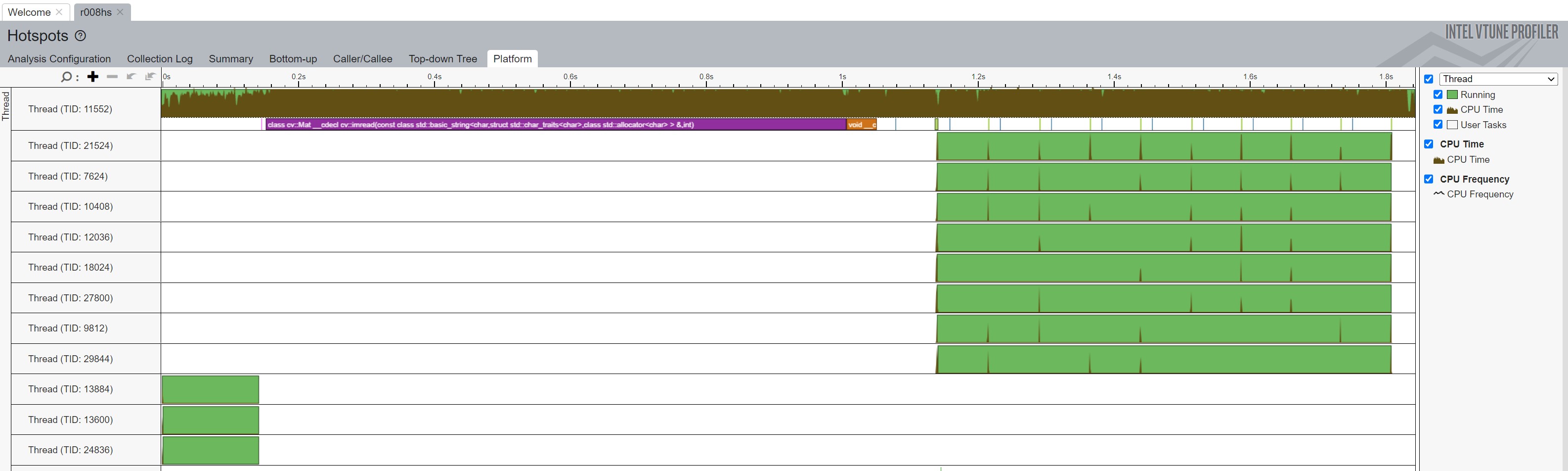
After executing and closing the program, VTune crunches all the information it has collected and presents various options for displaying it. In Figures 3 and 4, the Platform option was selected, and, as seen in the figures, VTune shows the number of operating threads and what portion of the code ran within each thread. In this case, both programs executed for 10 iterations which provides enough data for VTune to sample for trends. The initial zoom level provides a nice overview of the patterns of code execution. VTune also allows zooming in or hovering over the individual boxes to learn which method is represented by each box. However, even at this level of granularity the VTune plot for the Python code shows that twelve threads execute over the application's lifetime. The green areas represent times where the thread was running and the brown regions show where each thread utilizes the CPU.
The purple box in each figure represents the call to OpenCV's imread where the code loads the image to process. Note the scale along the top shows that in both cases the read takes around 1 second, they appear to be different sizes since the C++ graph takes 25 seconds while the Python graph completes in about 2 seconds.
To the right of the purple box represents the processing effort to extract the rectilinear image ten times. As shown in Figure 3, the C++ code utilizes a single thread, whereas, Figure 4 shows that the Python code distributes the work across eight threads. Ten brown spikes are visible for when each of those threads processes one of the ten rectilinear extractions.
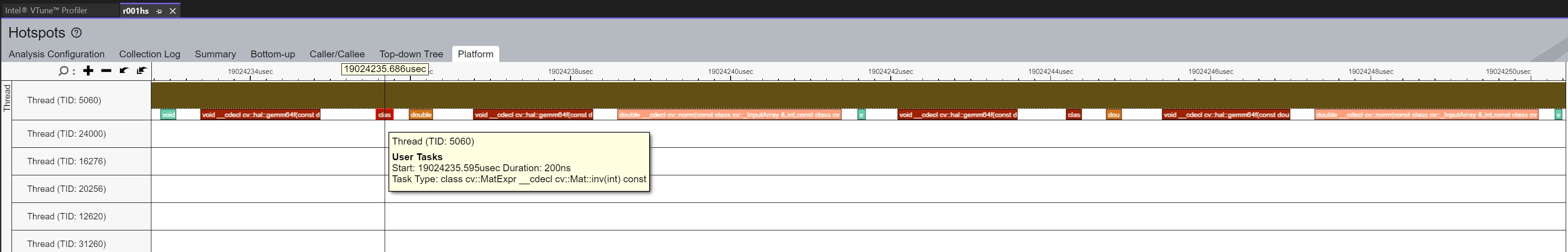
VTune enables a developer to zoom in on any portion of the execution to get more details on what code ran at any point in time. In Figure 5, the zoom level illustrates the individual OpenCV method calls made by the C++ code over a duration of about 17.5 microseconds. The tooltip shows that the method under the mouse cursor is the call to cv2.inv(). By hovering over each of the other function calls, VTune showcases that the code calls cv2's inv, then invert, gemm64f (a method to multiple matrices), norm (to normalize the xyz matrix), multiply (shown by the green box, which multiples the matrices), and finally gemm64f before the cycle repeats. The tooltip also shows the duration of each method call. For example, cv::Mat::inv executes for 200ns. The gemm64f tends to execute for around 1.5 microseconds, and cv::norm runs around 2.8 microseconds. While each call does not take a long time, it adds up quickly since these calls occur often as described in the summary page below.
These calls come from the code line in reprojection that looks like:
cv::Mat ray3d = Rot * K.inv() * xyz / norm(xyz);
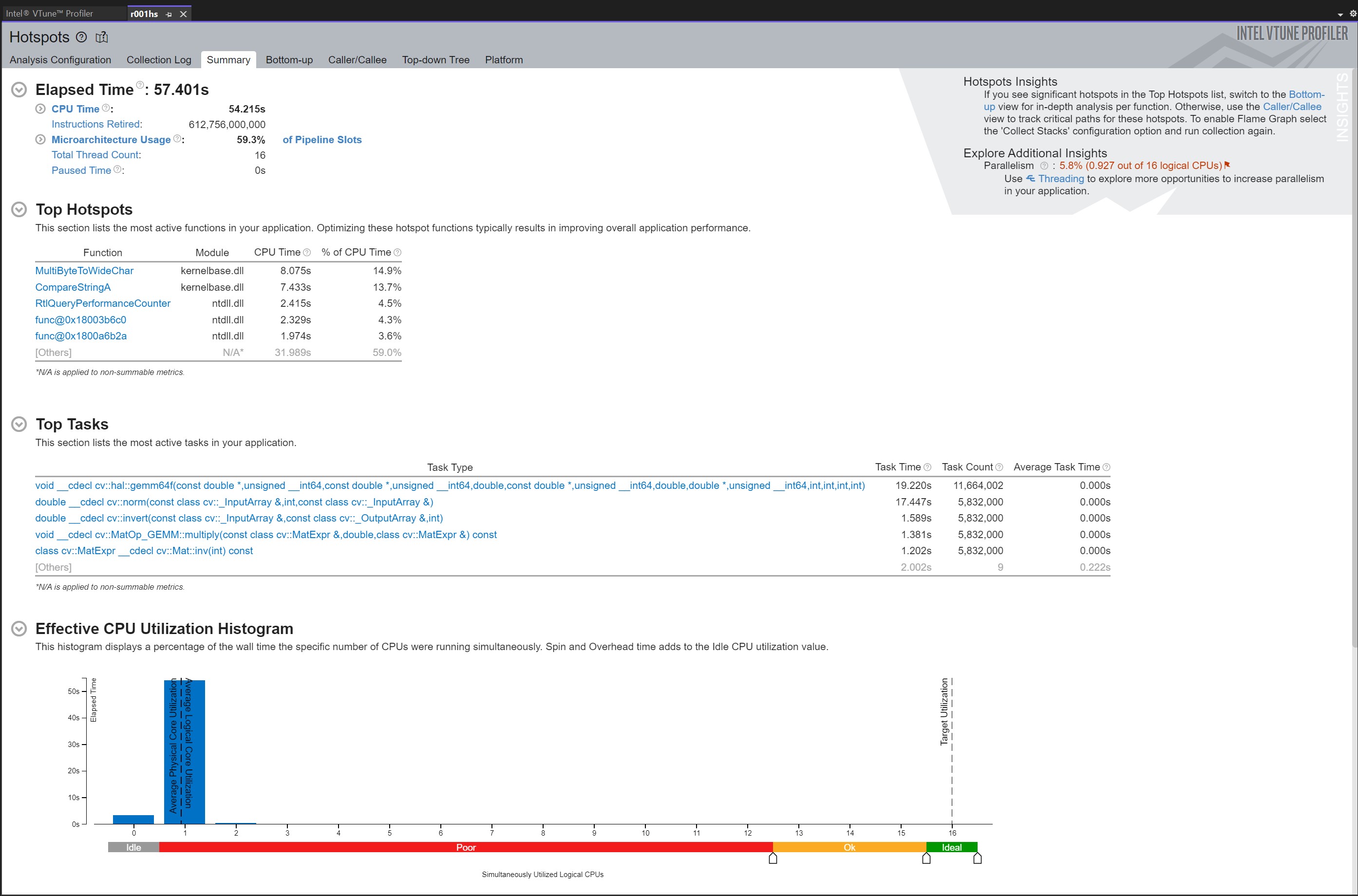
VTune also has a summary page shown in Figure 6. The Top Tasks section describes the most active tasks in the application. This reinforces that gemm64f, norm, invert, multiply, and inv are called many times, either 11.6 or 5.8 million calls, and account for much of the overall execution time.
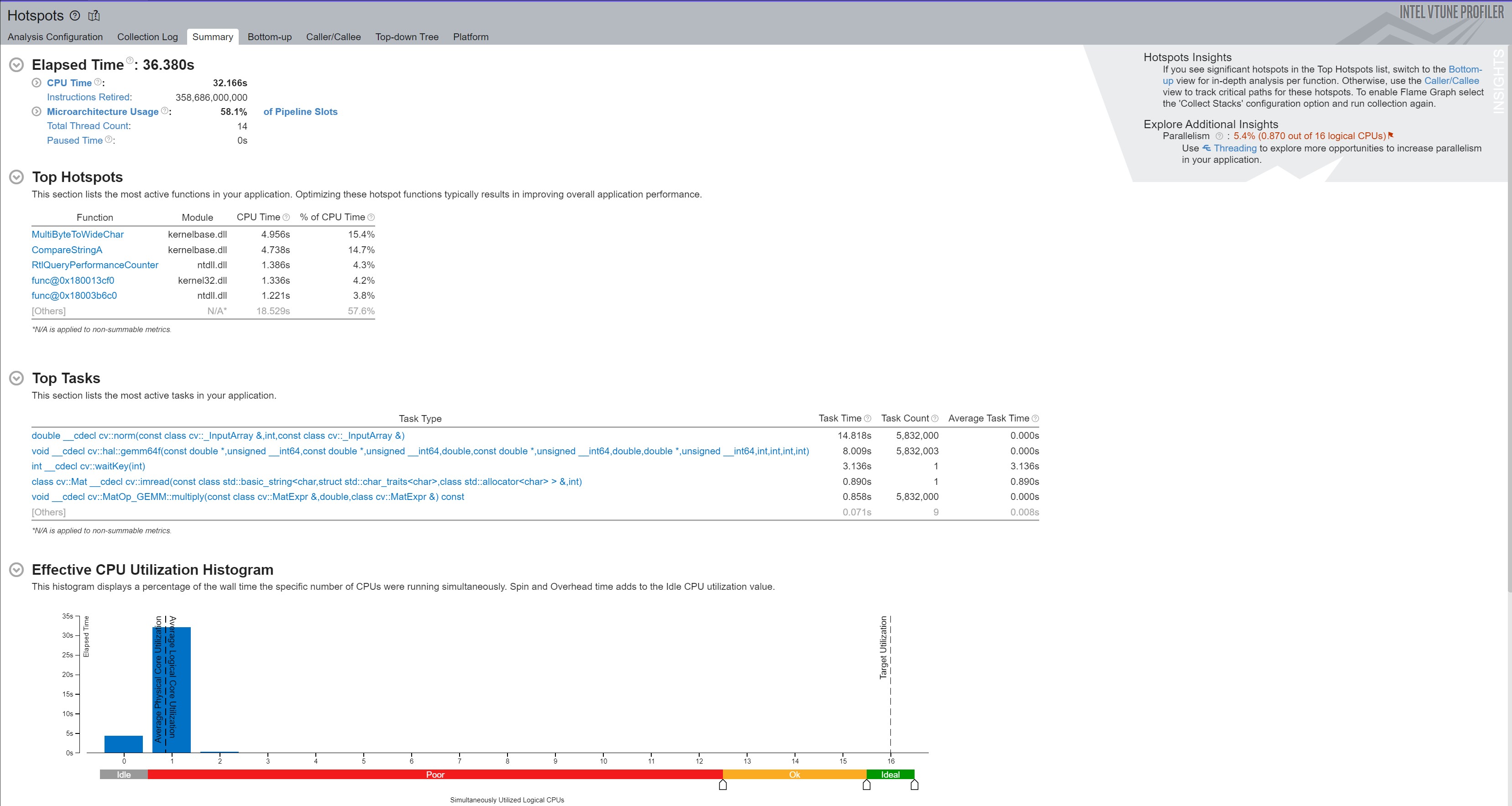
After inspecting the rest of the code, it becomes clear that Rot, K, and K.inv do not change over the call duration to bilinear_interpolation. Thus, the code can be optimized by computing Rot * K.inv() a single time (for example, in the constructor) and caching it for use in the reprojection method. Figure 7 shows the VTune summary of a code execution after caching. The results from running 100 iterations of the changed code, shown below, indicate the altered code executes about twice as fast (1.77149091 / 0.89846216 = 1.97), but still slower than the Python code. The speed-up comes from not making the extraneous calls to gemm64f, inv, and invert.
Release\equi2rect_example.exe # Original code Release mode
Average for 100 frames   1.11301293s   1113.01293ms  1113012.927us   0.89846216 FPS

Release\equi2rect_example.exe # Release mode - Cache Rot * K.inv()
Average for 100 frames   0.56449626s    564.49626ms   564496.264us   1.77149091 FPS
Due to some of the above limitations, the previous code could not be used for this blog series, which led to the creation a different JavaScript option. The Apache-2 licensed code can be viewed from https://intel-health.github.io/optimizing-equirectangular-conversion/1-Introduction%20to%20360%20Degree%20Representation/Equirectangular.js.
Loading the code requires adding the line:
<script type="text/javascript" src="Equirectangular.js"></script>
in the head region of an HTML page. Next, make the body line appear similar to this:
<body onLoad="displayFlattened([['../images/IMG_20230629_082736_00_095.jpg', 'PhotoFlattenedImage', 'PhotoRawImage']])">
The parameter to the function displayFlattened is an array of arrays to support multiple equirectangular images on one web page. In each sub-array the first element provides the URL for the image to load, the second element contains the canvas id where to place the flattened image, and the third element has the canvas id where to place the raw image. Both canvases must exist on the web page, but the display state can be set to none for the canvas elements that should not be seen by the user. By having both canvases, the web page can display either the rectilinear (flattened) view, the equirectangular (panoramic) view, or both. The Introduction to 360-Degree Videos and Imaging loads multiple equirectangular images and in some cases shows both views and, in some cases only, shows the rectilinear view. Use the View Page Source option to see all the details of how the Introduction web page was constructed.
Finally, on the web page create the canvas(es) to display the image(s) using HTML similar to the following and ensure the canvas id matches the id used when calling the displayFlattened function.
<canvas id="PhotoFlattenedImage" width="640" height="640" tabindex="1">
  Sorry, this browser does not support the HTML5 canvas element
</canvas>
This blog discussed some Open Source solutions and their advantages and disadvantages and introduced ways to measure the conversion speed when extracting the rectilinear view from a 360 panoramic image.
The next installment in the blog series, Execution Framework and Serial Code Optimizations, introduces a framework for testing different algorithm variations, continues exploring tools available to determine inefficiencies in the algorithms, and then proposes code changes to minimize the time for extracting a given field of view from an equirectangular frame. The efficiency assessments consider two cases: 1) where the field of view moves over an equirectangular image and 2) where the field of view stays in the same spot while the underlying image changes (for example, for working with a video stream).

|
Doug Bogia received his Ph.D. in computer science from the University of Illinois, Urbana-Champaign, and works at Intel Corporation. He enjoys photography, woodworking, programming, and optimizing solutions to run as fast as possible on a given piece of hardware. |
© Intel Corporation. Intel, the Intel logo, VTune, and other Intel marks are trademarks of Intel Corporation or its subsidiaries. Other names and brands may be claimed as the property of others.
The products described may contain design defects or errors known as errata which may cause the product to deviate from published specifications. Current characterized errata are available on request.